Stornoway System Optimisation

During the course of the modelling process, there where a few changes we had to make to achieve our initial aims. We had to remove the hourly operating reserve that was activated for a 10% change in the hourly load. This reduced our shortfalls to 0%, by dispatching power to meet the load instead of reserving it for an hourly change that might never occur.

We also designed a hydrogen fuel consumption schedule and operated the Fuel cell at a higher efficiency (i.e. 65.8%) to enable it meet the shortfalls created by the wind power system as a result of the intermittent nature of the wind resource.

Iteration was also applied during the modelling process to reduce the search space (which is a list of system configurations that the homer software considers for feasibility) and acquire the best configuration to meet our aims for this scenario.

Fuel Cell Optimisation

To guarantee the initial conditions for the fuel cell, a hydrogen load schedule had to be designed to consume Hydrogen efficiently. To simulate the Fuel cell at an electrical efficiency of 65.6% and the hydrogen load schedule, the following formula were used:

The first equation is used to plot the amount of Hydrogen consumed to produce electricity i.e. the fuel curve. The fuel consumption rate is F. However, as mentioned above we simulated the fuel cell system to run at 30% minimum load ratio as is evident from the graph (figure 1). The fuel cell system will shut off when the load is less than 30% of the Fuel cell system’s 4.5MW capacity.

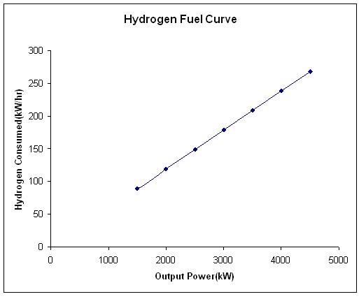
Fig. 1: Hydrogen Fuel Consumption Schedule

F0 is the fuel curve coefficient in kg/hr/kW, F1 is the fuel curve slope in kg/hr/kW. YGEN is the rated capacity of the fuel cell and PGEN is the power output of the fuel cell in kW.

The second equation is used to plot the efficiency curve. LHV is the lower heating value of hydrogen, which is the amount of energy released when hydrogen is combusted initially at 25 degrees Celsius and the by products are then returned to 150 degrees Celsius. The 3.6 Constant arises because 1kWh = 3.6MJ. Below, is the efficiency curve taken directly from the HOMER software.

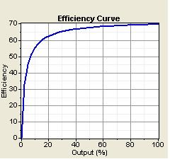
Fig. 8 Fuel Cell Efficiency Curve

The Fuel Cell System is simulated for full optimisation through out the period of one year. This means that the fuel cell system controls will not pre-empt periods of low wind speeds but will adjust the power output as is necessary to maintain a 100% power balance.